Appendices

APPENDIX A. DESCRIPTION OF THE GLOBAGRI-WRR MODEL

Overview of the Model

The GlobAgri-WRR model is a global agriculture and land-use accounting model. It estimates changes in agricultural production, greenhouse gas (GHG) emissions, and land-use demands over time, which result both from changes in demand for agricultural products and changes in production techniques, yields, and systems. Changes in demand may result from changes in population, diets, nonfood uses of crops such as biofuels, and levels of food loss and waste. Changes in production may result from changes in crop yields, livestock efficiencies or a broad range of changes in agricultural production methods. GlobAgri- WRR’s primary use is to estimate levels of land-use demand and GHG emissions at various points in the future, particularly 2050, and how various changes in demand or production methods might reduce those land-use requirements and emissions.

As an accounting model, the model estimates ultimate land-use requirements and emissions given a wide variety of parameters that are varied exogenously by the user or programmed into the model. For example, diets, populations, crop yields, nitrogen use efficiencies, and the intensity of livestock systems can all be varied, but the user must set exogenously to run the model for any particular scenario. The model is designed to answer questions such as what the changes will be in land-use requirements and total emissions, both from production methods and land use, if diets, populations, crop yields, and production systems in each country in 2050 follow certain estimates. It is therefore a means of estimating what set of demands and production systems would achieve environmental goals. In the course of doing so, the model also estimates many other parameters, such as nitrogen lost to the environment and changes in terrestrial carbon.

The initial drivers of the model are diets, population, and demand for nonfood agricultural products. The model is calibrated to match statistics from the Food and Agriculture Organization of the United Nations (FAO) for the reference year of 2010 using an average of 2009–11 to avoid overreliance on the results of a single year. These statistics include diets at the country level (set forth in FAO food balance sheets),1 production, harvested area, cropland, and pasture. Food loss and waste rates are based primarily on a 2011 FAO study,2 which GlobAgri-WRR adjusts to reflect estimates of processing and transformation losses in FAO food balance sheet data and thereby avoid any double-counting between the 2011 FAO study and the FAO food balance sheets.

The reference year inputs are disaggregated at the country level, including not just demands but the various coefficients that translate demand for agricultural products into production, inputs, and land use, such as levels of waste, calorie balances, and livestock production systems. When the model is “run,” which involves solving for trade and some other interactions among countries, these levels are aggregated to a regional level both to avoid excess computation requirements and to smooth out possible data errors at the country level. When coefficients for parameters are missing at the country level, regional estimates are assigned to each country within the region.

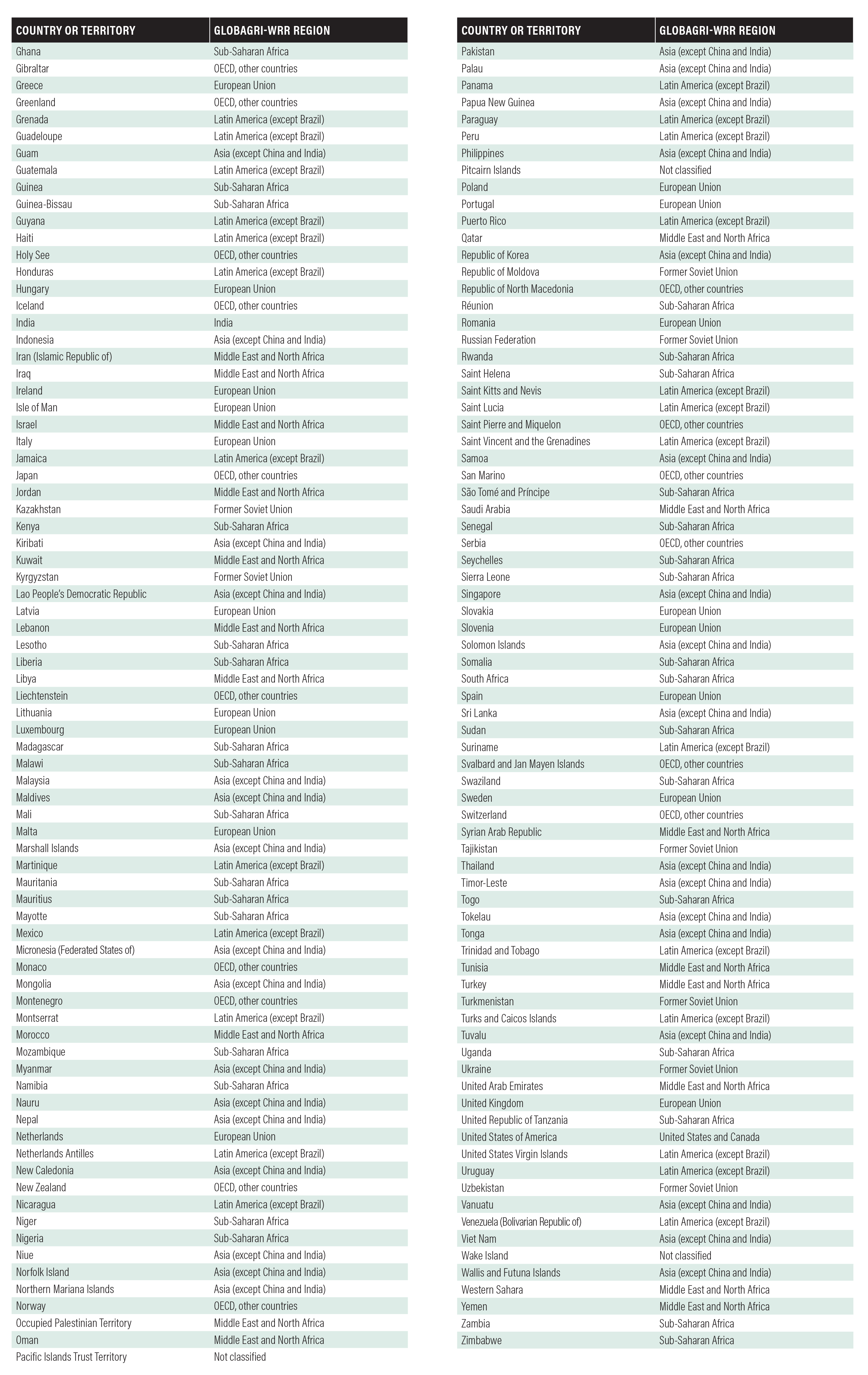
Overall, the model can estimate how changes in population, diets, other crop demands, rates of losses and wastes, and/or production techniques within any one country will change production, emissions, and land-use demands regionally and globally. Table A-1 shows how the world’s countries and territories are grouped into 11 regions in GlobAgri-WRR: Asia (except China and India), Brazil, China, European Union, Former Soviet Union, India, Latin America (except Brazil), Middle East and North Africa, Organisation for Economic Co-operation and Development (OECD, other countries), sub-Saharan Africa, and the United States and Canada. Because the regional disaggregation is fully flexible, it is also possible to use any individual country as a region, and in the standard operation of the model, Brazil, India, and China are both countries and regions.

At the country level, the model works with the 117 agricultural products that are a part of FAOSTAT commodity balance levels. For specific purposes, in particular trade and nitrogen balances, some products may be further disaggregated into finer agricultural products, which FAO calls supply and utilization account (SUA) commodities. For example, pulses are divided into separate types of beans, and the category of vegetables is divided into separate vegetable products. This further disaggregation is used to analyze trade because FAO reports trade in these products at more detailed levels, and to determine nitrogen contents of crops in order to estimate nitrogen surpluses. By contrast, some derived products are merged with the product they are derived from using energy equivalent quantities and after accounting for processing losses. For example, demand for a certain quantity of beer results in demand for barley with equivalent energy content after accounting for transformation losses.

Although these country-level products are used to calculate land-use demands, GHG emissions, inputs, and other factors, all interactions among countries occur at the regional level both to reduce processing time and to smooth out errors in data that may occur at the country level for some products. In addition, to limit processing time, the more detailed agricultural products are aggregated to 33 product aggregates at this regional level. Some of these aggregates remain as unique products, as is the case for wheat, maize, rice, soybeans, soybean oil, soybean cakes, beef, dairy, and eggs. Feed products not in commodity balances are also included at both the country and regional levels, most prominently grass. For the most part, country-level and commodity-balances parameters can be individually varied, allowing the model to compute model inputs using whatever detail is available at the country and detailed products level.

Table A-1 |

Countries, territories, and regions in the GlobAgri-WRR model

Note

The European Union comprised 27 member states in 2010, the base year used in the model.

Although the core of the model is an elaborate accounting system, the model incorporates results from a variety of submodels that use a range of biophysical processes to estimate emissions or the relationship of inputs to production. These models include the following, which are discussed in further detail below: .

• Land use: A model to estimate the source of new agricultural lands by region and resulting GHG emissions from land-use change developed primarily by researchers at the European Commission’s Joint Research Centre.
• Livestock: A model estimating representative production systems, feeds, and emissions at the regional level for beef, milk, sheep and goats, pork, chicken, and eggs developed primarily by researchers at the Commonwealth Scientific and Industrial Research Organisation and the International Institute for Applied Systems Analysis.
• Aquaculture: A model to separate aquaculture production by representative production systems within major producing countries or regions, and to estimate land-use demands, feed requirements, and emissions developed by WorldFish.
• Rice: A model to estimate GHG emissions from rice production developed primarily by a researcher at the Institute for Soil Science in Nanjing, China.
• Nitrogen: A model to estimate nitrogen demand and emissions by different crop types and country developed primarily by researchers at Princeton University.
• Energy use: Estimates of emissions from agricultural energy use developed by the U.S. Environmental Protection Agency and by FAO.

Categories of Agricultural Products

The model manages three types of agricultural products:

1. Primary vegetal products, such as wheat, soybeans, or grasses, are grown on land. Based on levels of demand, location or production, and yield, the demands for these products translate into demand for cropland and/or grazing land (and, based on production techniques, into GHG emissions). Demand for these products may be direct, or it may result from demand for transformed products, such as meat. At the regional level, the model aggregates the primary vegetable products into 15 categories of primary vegetal products based on commodity-balances products and three grass products.
2. Transformed products provide a second type of product demand, including vegetable oil, oilseed cakes (sometimes called meals) used for livestock, biofuels, alcohol, and various meats, milk, and eggs. Some of these products are in direct demand, such as the demand for meat and milk or vegetable oil. The demand for some others, such as oilseed cakes, which are used as an animal feed, derives from demand for other products, such as meats and milk, and may depend not only on their levels of demand but also on production systems specified in the model. For example, the amount of soybean cake required will depend not only on the quantity of various livestock products but also on the production systems specified for those products. There are 17 such products at the regional level.
3. The third type of agricultural product does not require land, directly or indirectly. It corresponds to aquatic plant, honey, game, and other such products but also to some livestock by-products, such as offal. These products play a small role, and when diets or livestock production systems call for such products, the model generates them without emissions or land-use costs.

The report refers to “animal-based foods” (and subcategories of such foods) extensively throughout Chapter 6—which are a combination of the second and third types of agricultural products noted above. See Figure A-1 for additional clarification about the different subcategories of animal-based foods modeled in this report.

In each case, the model also uses FAO data to relate calories available as food in each region and country to food quantities produced based on commodity-balance food products information included in food balance sheets. These coefficients vary by country because FAO estimates of the calorie content of final food products differ from country to country (mostly modestly but sometimes to a large degree) and because final products differ in quality and type (for example, the type of beef consumed). The calories-to-quantity coefficients must reflect these different calorie contents. For products that are the result of processing (e.g., alcohol), the relationship of production to consumption must also reflect losses during processing. We describe in more detail how those coefficients are calculated for processed products below.

Overall, one feature of this model that differs from most or all previous global agricultural models is the higher degree of disaggregation into both different food products and their transformed products. This makes it possible to analyze changes in more detailed diets.

Model Computational Structure

For the most part, the model works like a series of interlocked spreadsheets translating demand for all types of agricultural products into production in different countries and calculating the land use and other inputs required for that production and, from these inputs, the emissions generated during that production. In certain features, however, the model must resolve demand and supply through more complicated algorithms.

Trade

In the base year, imports and exports are specified by FAO data at the country level and aggregated to the regional level using FAO bilateral trade information to remove intraregional trade. From these data, each region’s “dependence ratio” and “share in global gross exports” are calculated for each agricultural product. The dependence ratio is the ratio of a region’s gross imports divided by the region’s demand for domestic consumption. If a region has gross imports of 10 units and consumes 100 units of a product, its dependence ratio is therefore 10 percent. The “share in gross exports” is that country’s share of global gross exports. If
a country contributes 20 units of total gross exports of a product among all exporting countries, and the world’s total trade of that product is 100 units, that  country’s share in gross exports is 20 percent. 

In future scenarios, the baseline assumption preserves both the “dependence ratio” and the “share in gross exports.” A region may both import some of the same product and export that product, in general because of different types or qualities of a crop or agricultural product. This system preserves both roles in global markets. To explore future scenarios, the model can be run with different trade shares and dependence ratios.

Figure A-1 |

Animal-based foods are split into eight categories in the GlobAgri-WRR model

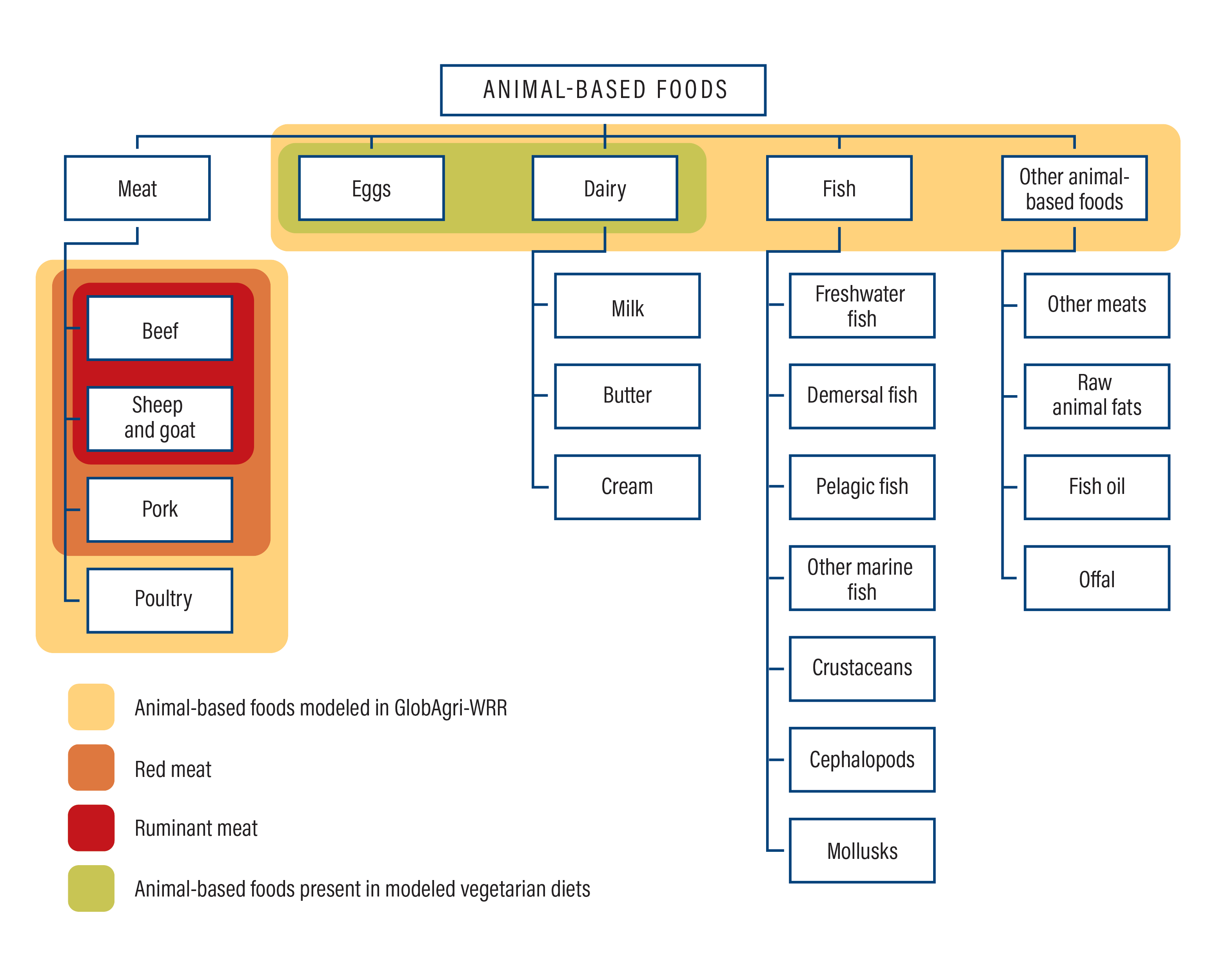
Note

Offal refers to the entrails and internal organs of an animal used as food. Demersal fish refers to fish living near the floor of a body of water. Pelagic fish refers to fish that exist in the pelagic zone of a body of water, which is neither close to the shore nor close to the bottom. Cephalopods refers to sea life with prominent heads and tentacles, such as squid and octopi.

Source

GlobAgri-WRR model and FAO (2019a).

Land Use 

In some scenarios that the model could analyze, there are possibilities for increasing agricultural land-use demands within a country to levels in excess of available land. To avoid this scenario, when a country runs out of agricultural land, the model is programmed to cap production and to meet rising demand by changes in net imports. This cap would only become relevant for extremely high growth scenarios.

We also have special rules regarding dry grazing land. In general, the model assumes that the full range of global production systems meet milk or meat demands in the base year. However, we believe that all or virtually all dry grazing land available in a country is used today, so that increases in grassland areas must come from wetter systems (humid or temperate). We also believe that because dry grazing lands have little alternative use, they would continue to be used even if demand for milk or ruminant meat declined. We therefore program the model so that changes in supply of milk or ruminant meat do not come from  increases or decreases in arid grazing systems and instead result in changes in humid and temperate production systems.

By-products, Processing Products, and Coproducts

We take diet consumption in the reference year from FAO commodity balances. FAO reports these data per country. These balance sheets cover a wide variety of products that are derived products, such as sugar and sweeteners, alcohol, vegetable oils and cakes, brans, milled rice, and milk and meats. In addition, some products may be joint products. For example, soybeans generate both soybean oil and cake, and producing milk will result in both milk and some meat production. It is possible to handle these transitions by translating all final products into primary product equivalents. For example, a kilogram of soybean oil can be transformed into a fraction of a kilogram of soybean crop that might correspond to its weight or calorie percentage. An advantage of this approach is that it limits the number of products, and also implicitly accounts for changes in coproduct shares when demand changes. But a limitation of this approach is that the quantities of processed products may not be physically possible. For example, the percentages of soybean cake and soybean oil consumed may be different from the physical quantities actually produced by a given quantity of soybeans. In part because of the growing dietary importance of vegetable oil, which may come from multiple sources, we wished to have a model that was physically possible for those products. We also wanted to have primary equivalents for other products—namely, sugar and sweeteners, alcohols, and brans. The model therefore establishes rules so that production of a primary product is driven by its largest coproduct by energy value—for example, soybean cake in the case of soybean products. The quantity of soybean oil production is therefore established by the demand for soybean cake for animal feed.

Similarly, the FAO commodity balances show that many products (e.g.,crops) are devoted to processing. The finished products that come out,such as alcohol, may derive from different combinations of primary products, such as different grains. During the processing, some product quantities are also lost or transformed into bran and some other products that are typically used for animal feed and that do not show up in food balance sheets. The commodity balances do not directly permit a mapping of processed products to primary products, and such a mapping is not straightforward. One challenge is that FAO estimates of calorie contents of food calories vary by region or country (e.g., a kilogram of beef will have different calories in one country compared to another because the types of beef products are considered to vary). Ultimately, consumed calories in the different product categories have to map consistently and plausibly to primary  products, both produced domestically and imported.

Programming in GlobAgri-WRR is designed to address these challenges in a variety of ways. For derived products, such as raw sugar, sweeteners, alcohols, and brans that can be derived from diverse products, we first determine the relative contributions of different processed inputs. There could be more than one solution for the determination of a derived product source. For example, wheat and maize processed in alcohol and sweeteners may be combined in different ways. As one example, all the sweeteners may come from maize and the remaining processed maize could be used as alcohol, then processed wheat  would be used to produce the remaining alcohol. However, many other combinations are possible. We use a minimization to find a unique solution by trying to keep the share of input product in derived product similar to the share of processed use in total processed uses for corresponding products. In the example above, if processed maize is twice as high as processed wheat, then two-thirds of alcohol and sweetener will come from maize and one-third from wheat. This calculation is done only for the reference year to set coefficients for the model in general.

Finally, for derived products set forth in use by FAO that are not explicit (brans, sugar, alcohols), we compute the transformation coefficients so that primary products and ultimate products are equivalent. For example, if diets report consumption of alcohol, and some of that alcohol is imported, these demands and imports are transformed into primary products both for calculating diets and imports. All the computations described above concern commodity balances products and reference year balances and coefficients. Turning to the model resolution, for sugar, brans, and alcohols, all the demands for food and feed are translated into primary products demands, mostly cereals and sugar crops. The model resolution is therefore simple for those products.

For oil and cakes that are joint products of oil crops and meat and milk that are joint products of the dairy sector, a different approach must be used to assure physical consistencies for the reasons discussed above. In the case of oil crops except for oil palm fruit, the quantity demanded is based on the quantity of oilseed cakes required. The oil is treated as a by-product and is the first source of vegetable oil. If more vegetable oil is required, the model estimates that this supply will comefrom palm oil production because it is the cheapest source of global vegetable oil production. For this assumption to function, palm kernel cake and palm oil are considered to be produced independently so that palm oil demand can be met by increased oil palm production without  increasing production of palm kernel cake. Similarly, the quantity of meat produced by the dairy sector depends entirely on the quantity of milk demand, with the meat treated as a coproduct. The remaining meat demand is filled by production systems for beef or small ruminant meat that produce only meat.

Aquaculture

In the case of aquaculture, the model determines feed available from fish (a composite of oil and meal) as a percentage of available wild fish consumption. Because the wild fish harvest has not grown for more than 20 years, we do not believe any additional wild fish consumption is possible and therefore cap the level of fish and fish feed at 2010 levels. We have rules to ensure that additional aquaculture production substitutes oilseeds for wild fish. (For some years, diversion of fish feed from other livestock products may serve as the direct source of additional aquaculture production, but that would require additional consumption of oilseeds by other livestock sectors with the same net result.)

Waste

FAO food balance sheet data provide a category of waste for uses of food, but the category is too small to account for all sources of waste. GlobAgri-WRR therefore incorporates estimates of waste for each product in each region from FAO (2011c). To avoid double-counting waste, we add “waste” in FAOSTAT back into the food available for consumption and then use loss and waste coefficients from FAO (2011c). Because FAOSTAT food balance sheets already assume transformation losses in food that goes through processing, we also do not include “processing and packaging” wastes estimated in FAO (2011c). “Postharvest handling and storage” losses going through local food systems are also accounted for. The result should be actual diets.

One of the issues with FAOSTAT and FAO (2011c) estimates of waste is that resulting actual diets appear likely to remain substantially higher than the calories people probably eat. As reported in Del Gobbo et al. (2015),3 there is a large discrepancy between the calories FAO data imply that people actually consume even after adjusting for loss and waste estimates, and the calories that people claim to eat based on food surveys around the world. For example, U.S. Department of Agriculture (USDA) food surveys claim that people in the United States on average consumed 2,081 calories per day in 2009–10. By contrast, FAO food balance sheets, which are also based on USDA data, estimate food availability of 3,711 calories per person per day, which according to our calculations translates into 2,922 calories per person per day after adjusting for estimates of waste in the retail and consumer sectors. This difference is part of a broader set of discrepancies. For example, Del Gobbo et al. (2015) found that while the FAO balance sheets estimated much higher food availability than consumption for most foods, they typically underestimated reported consumption of beans and legumes and nuts and seeds.

These discrepancies lack a full explanation. They may represent overestimates of food available by FAO, but they may also reveal underestimates of food consumption by people responding to surveys. One possible explanation for the underestimate of nuts and beans is that FAO may be failing to count some home production or wild-gathered nuts and seeds. Another possibility is that the FAO (2011c) estimates of food losses and waste, as high as they are, underestimate actual food waste, particularly if they fail to count portions of products that many people don’t ultimately consume but may not consider waste (such as the interior parts of vegetables, or the fattier parts of meat, that the affluent throw away). For purposes of GlobAgri-WRR, what is most important is that the land (and chemicals) used for agricultural production ultimately correspond properly to diets. If losses and wastes are higher than otherwise estimated in FAO (2011c) and consumption is lower, this relationship between land and inputs and diets will remain accurate. At this time, there is no alternative to using FAO data for this type of analysis.

Land-Use Requirements

The model specifies a production level for each crop and for livestock in each country based on demand and trade. Land area requirements for each crop are then based on specified yields and cropping intensities, which reflects the ratio of total cropland area to harvest. The model uses an average cropping intensity for all crops within a country. These figures are based on FAO data in the reference year. In future years, yields and cropping intensities can be specified as a model input.

For grazing area, the model computes a demand for grazing area forage from the livestock module and in the reference year, an average yield of forage per hectare of grazing land in each of several climate zones. Forage quantities from grazing land are based on the model used for Herrero et al. (2013), discussed below. Grazing areas per climate zone were based on an overlay of the zones as specified by FAOSTAT and maps of grazing area from Bouwman et al. (2006). The climate zones are arid, humid, and temperate within each country. For reasons discussed above, all growth and reductions in livestock grazing areas in future years are estimated to come from humid and temperate zones. Grass yields are therefore specific to those zones. For future years, the model permits specification of percentage changes in grassland yields. Increases in tons of grass consumed per hectare could result either from improved grass growth or more efficient grazing, and the model does not differentiate. (The livestock model also permits specification of improved livestock yields due to more efficient conversion of feed to meat and milk, but that improvement is made through the livestock module.)

Emissions

The model focuses on emissions up to the farm gate, including emissions involved in the production of farm inputs. Emissions from land-use change are also calculated separately and can be combined with production emissions.

Emissions are based on carbon dioxide, nitrous oxide, and methane (and do not include other pollutants such as black carbon and aerosols, or impacts on climate through tropospheric ozone or changes in albedo). In all cases, emissions are counted both in their actual gasses and using global warming potential (GWP) for 100 years. To calculate the GWP of 1 kg of methane, the model uses 34 kg of carbon dioxide equivalent based on the recommendations of the most recent comprehensive assessment of the Intergovernmental Panel on Climate Change (IPCC). These figures contrast with a GWP 100 of methane of 25 under the IPCC’s 2006 national reporting guidelines, which most countries and international institutions still use. The GWP 100 of nitrous oxide is 298.

The model computes the following categories of GHG emissions in ways that incorporate several other models as follows:

Livestock emissions (enteric, manure management, and paddocks, range and pasture)

The model estimates both emissions from livestock and types and quantities of feed required using a representation of livestock systems used in Herrero et al. (2013). As part of that exercise, the authors separated the world’s ruminant livestock systems into 27 regions, and in each region, into up to eight representative systems based on the Sere- Steinfeld livestock categorization system. Those systems are based on grazing-only systems, mixed systems (combining some grazing and some confined feeding), and “urban,” which are entirely confined systems. Grazing and mixed systems were also grouped into arid, humid, and temperate zones, which include tropical highlands. Ruminant systems were also categorized as bovine dairy, bovine meat, small ruminant dairy (sheep and goats), or small ruminant meat. For each system, the team estimated average feed diets and dominant breeds used, and basic herd characteristics (such as fertility and mortality rates). The team then estimated production using the “ruminant model,” which is a biophysical model developed by Herrero that simulates ruminant digestion, energy and protein uptake, and their translation through different cow breeds into live weight gain and milk production. The model is sensitive to the precise qualities of animal feeds. Using a number of convergence algorithms, the modelers adjusted the estimates to fit FAO data for livestock numbers, production, and animal feeds tracked by FAO.

The model calculates feed requirements in the following categories: crops, forage from grazing land, forage characterized as “occasional” (forage gathered by cut and carry systems or wastes from agricultural processing), and “stover” (crop residues). (The underlying model also uses types of stover and wastes.) Crops in turn are segregated into barley, corn, pulses, rice, sorghum and millet, soybeans, wheat, other cereals, other oil seeds, canola, and feed from animal products.

Running GlobAgri-WRR does not require running ruminant or the underlying herd model but instead incorporates these results based on the regions and production systems. For each production system, the model incorporates the estimates of feed requirements per kilogram of production and emissions generated per kilogram of production. For the reference year, the model allocates ruminant production in a country to the different systems in proportion to the regional distribution of livestock systems’ grass demand estimated by Herrero et al. (2013) for the year 2000, using system-specific grassland areas in countries and regional system grassland yields. For monogastrics, the regional system production shares are used to split country production in the different systems. The quantity of production otherwise calculated by GlobAgri-WRR in a region or country, multiplied by share of a production system, and multiplied by either the feed requirements or GHG emissions per unit of production for that system generates the total feed requirements and emissions in total for that system. GlobAgri-WRR then sums these feed requirements to the national or regional level, where they determine the production of feeds and trade. GlobAgri-WRR also sums the emissions to the global level.

The ruminant model embedded in this livestock system estimates both methane emissions and the nitrogen content of wastes. Based on system, the overall model estimates the portion of this nitrogen that is deposited on paddocks, range, and pasture (PRP) and the portion that is subject to a form of concentrated manure management. The model then uses Tier 1 coefficients from the IPCC 2006 national GHG reporting guidelines to estimate emissions from nitrous oxide associated with these nitrogen excretions. The ruminant model also estimates quantities of waste. The overlay model determines the manure management system for those systems that involve concentrated production of manure and uses Tier 1 IPCC emissions factors for that management system to estimate methane emissions.

The same paper also generates analyses for pork and poultry systems, divided between egg production and meat. Within each region, pork and poultry production are divided between intensive (“urban”) and extensive (“other”). Only crop feeds are individually listed, as other feeds are considered to be wastes and residues of some unspecified type. The authors estimated waste management systems by region. Emissions are based on Tier 1 methods from the IPCC 2006 guidelines.

For future years, GlobAgri-WRR can be run through variations on these livestock systems by estimating changes in the mix of livestock systems within a region or by introducing improvements in livestock systems whose effects are separately estimated using the ruminant model and herd model to generate emissions and feed requirement estimates.

More details about the livestock model components, including a description of the ruminant model, are presented in the published online supplement to Herrero et al. (2013).

Rice methane emissions

Rice methane emissions are based on the model developed and presented in Yan et al. (2009) based on IPCC 2006 methods. According to these methods, rice production from irrigated fields is influenced by the length of period of flooding within the cultivation season, the flooding regime outside of the cultivation period, the types of soil amendments added (particularly crop residues), and whether the in-season flooding is continuous, interrupted once by a drawdown that allows oxygen to penetrate soils, or interrupted by multiple drawdowns. Yan et al. (2009) developed a spreadsheet model based on understanding of these conditions in the rice-growing countries, and which allows for changes in water management conditions and soil amendments. The model can produce average national estimated methane emissions for each hectare of rice production. GlobAgri-WRR incorporates these estimates for the baseline year based on the model per country. For future scenarios, the rice model can be run “off-line” to estimate changes in these average national emissions based on changes in management practices. Such changes can then be incorporated as part of mitigation scenarios.

For this process, we made one change to the version of the model used in Yan et al. (2009). The version for that model built in assumptions of very high levels of single and multiple drawdowns across the world’s irrigated rice production based on figures provided in an Asian Development Bank report. These estimates seemed too high to the authors of the World Resources Report rice installment in Adhya et al. (2014). We adjusted these estimates so that one midseason drawdown is assumed to be common only in Japan, China, and South Korea (90 percent of irrigated production), and there is no meaningful rate of multiple drawdowns. In all other countries, only 10 percent of irrigated production is estimated to experience one midseason drawdown.

Nitrogen fertilizer use and nitrous oxide emissions

Nitrous oxide emissions from agricultural soils are a function of all nitrogen applied to soils whether from fertilizer, nitrogen applied in manure, nitrogen deposited on soils by grazing cows, nitrogen fixed or absorbed by crops and left in crop residues, or nitrogen deposition. For cropland and for the portion of nitrogen applied to pasture from fertilizer, the model is now programmed primarily to generate emissions using an IPCC Tier 1 emission factor for direct and indirect nitrous oxide emissions of 1.425 percent of applied nitrogen. An exception is that nitrogen for irrigated rice production is based on the IPCC emission factor of 0.3 percent, because of the extensive evidence that flooding reduces nitrous oxide emissions. The model can easily be run using alternative emissions coefficients. The model can also estimate nitrous oxide emissions based on nitrogen surplus (the excess of applied nitrogen over nitrogen removed in crops, according to a formula estimated by van Groenigen et al. 2010).

Total nitrogen application rates, including nitrogen from synthetic fertilizer, manure, biological nitrogen fixation, and nitrogen deposition, are based on a database presented in Zhang et al. (2015b) and described in its supplement. This database was developed using data from a variety of sources, with particular reliance on data sets established by the International Fertilizer Association (IFA) and FAO. The nitrogen database in Zhang et al. (2015b) provides estimates on nitrogen input rate from four different sources, namely fertilizer, manure, biological nitrogen fixation, and deposition, by country and crop type for the period 1961–2011. The database covers 153 crop types and over 190 countries, which account for more than 99 percent of the global total nitrogen input to cropland. The nitrogen fertilization rates are estimated based on reports by IFA and FAO on fertilization rates by country and crop types for recent years (namely, 2000, 2006, 2007, and 2010). Nitrogen deposition rates for each country and crop type are estimated based on maps of nitrogen deposition and crop distribution. The projected deposition rates in 2050 are estimated based on the projection in Bouwman et al. (2013) and the crop distribution map around year 2000. Nitrogen fixation rates by leguminous crops are estimated based on the crop type and yield following methodologies used in Van Grinsven et al. (2015).

In addition, this database provides information on nitrogen removed from cropland in the form of food product, and consequently the nitrogen use efficiency (NUE) by crop type and country (or region), which is defined as the ratio of nitrogen removed by harvested crops divided by total nitrogen inputs. Along with nitrogen inputs from other sources, fertilizer demand can be estimated over time as a function of NUE, crop production, and crop yields. By estimating changes in NUE, various potential mitigation options can be analyzed.

For nitrogen from manure, to ensure consistency with the livestock model and potential changes in livestock production, we replaced the manure estimates in Zhang et al. (2015b) with manure estimates from the livestock model adapted from Herrero et al. (2013). In addition, because nitrogen in crop residues is not explicitly accounted for, a coefficient is used that links nitrous oxide emissions from residues to other sources of nitrous oxide emissions based on FAOSTAT emissions data.

Energy Use

Energy use emissions come from two categories: energy used on farms to run machinery, and energy used to produce fertilizer and pesticide inputs. Emissions for energy use on farms are taken from FAOSTAT and are assigned within a country by hectare of harvested area. Emissions for pesticides are based on quantities of pesticides used by hectare and country using the same methodology as the U.S. Environmental Protection Agency (EPA) for a 2009 rulemaking for the Renewable Fuels Standard expressed in a worksheet included in the docket for a rulemaking published on March 26, 2010, titled EPA-HQ-OAR-2005-0161- 3175.17.4 The analysis also includes estimated emissions and quantities for the production of phosphorus, potash, and potassium, which are also estimated per hectare for each of 11 crop types using IFA data. For nitrogen use, the model uses the nitrogen model subcomponent to estimate quantities of synthetic nitrogen used and then estimated emissions factors associated with synthetic nitrogen synthesis from the EPA document.

Land-Use Emissions

Emissions from land-use change are based on a model developed by researchers at the European Commission Joint Research Centre (JRC), originally described in Hiederer et al. (2010). This land-use model estimates the quantity of GHG emissions that will be generated by land-use change for a specified quantity of hectares of a particular type of crop within a specific region. It does so by identifying existing croplands and areas devoted to specific crops (Ramankutty et al. 2008; Monfreda et al. 2008) and identifying potentially suitable land for each specific crop that is not in crop production from the GAEZ/FAO model, and then a variety of mapped products to identify different landscape types. After excluding land within a cell that is not suitable for production of a particular crop, the model then selects lands within a cell that are not cropland. In each cell with crops of any particular type, the assumption is that cropland expands into remaining ecosystem types in proportion to those types. This analysis is based on an assumption but grounded in extensive empirical evidence that agricultural expansion tends to work outward from existing agricultural areas.

Expansion of cropland results in levels of vegetation and soil carbon stocks falling from those found under natural vegetation to those found under cropping systems. To estimate carbon stocks, the model uses vegetative carbon stocks based on the IPCC 2006 default values for different ecosystems as synthesized in the guideline for the European Commission Directive on Renewable Energy (European Commission 2010). The IPCC provides values for a broader range of ecosystems than our five land-use categories.5 The JRC model uses these different land-use categories to estimate carbon stocks and changes but groups changes into five broader land-use categories: open forest (less than 30 percent canopy cover), closed forest (30 percent to 100 percent canopy cover), scrubland (woody plants lower than 5 meters not having clear aspects of trees), grassland, and sparse vegetation. Soil carbon stocks within the top meter were estimated based on the Harmonized Soil and Water Database (version 1.1).6 The GlobAgri-WRR model assumes that cropland conversion causes the loss of one quarter of soil carbon from the top meter, while conversion to grazing land does not alter soil carbon stocks.

In GlobAgri-WRR, the quantity of grazing land is dictated by demand for livestock and livestock systems. If the JRC model estimates that cropland would expand into grassland used for grazing, the area of grazing land would have to expand further. The JRC model can also be run to estimate land-use types converted for grazing. When the model estimates that cropland would expand on to grazing land, we therefore substitute for that grazing land a mix of land-use types that would be converted for expanded grazing. Because little of the world’s true native grassland (as opposed to scrubland or woody savanna) is not already used for grazing, we assume that all grassland conversion for crops reduces grazing land and therefore triggers this second-order conversion to replace the grazing land. This second-order conversion comes from ecosystem types that the model estimates would supply new grazing land in proportions based on the cell-by-cell analysis, but those sources of potential grazing land are restricted by GlobAgri-WRR to scrublands, open forest, and closed forest on the grounds that existing native grazing land is already used.

These calculations result in average carbon emissions for each hectare of land expansion in each country for pasture or for each type of crop. The central features of GlobAgri-WRR use these estimated emissions rates per hectare if the model estimates a change in demand for a type of crop or pasture within a country. Although the precise rate of emissions per hectare varies for each run of the model, typical average conversion rates for global changes in diets are around 85 tons of carbon per hectare, including both vegetation and soil carbon. These average emission factors are slightly higher than the average emissions per hectare used by the U.S. EPA for biofuel regulations (for the 2017 case) of roughly 76 tons of carbon per hectare.7 One likely reason is that the EPA analysis used an international model focused on cropland expansion, which did not require that all converted grazing land be replaced. As a result, substantial areas of relatively low-carbon grazing land could be converted to crops without any further conversion of higher-carbon forest and savanna. Under the accounting approach in GlobAgri-WRR, a reduction in grazing land due to crop conversion requires an increase in pasture area for the same level of production, and this pasture land requires a further conversion of savanna, scrubland, or open or closed forest. All net increases in agricultural land can therefore only come from these land covers. The EPA model also did not account for the high carbon losses associated with peatland conversion for palm oil production in Southeast Asia.

One challenge in calculating emissions from land-use change is that methods such as those employed by our model typically ignore the forgone carbon sequestration that would occur in forests, and some savannas and scrublands, if the land were not converted to agriculture. Carbon stock estimates are typically based on existing forests, not undisturbed forests. Many and probably most of the world’s forests and woodland/savannas have been subject to forest harvest, whether for commercial production or firewood, and have depleted carbon levels. In satellite mapping systems, many lands that appear as savannas and open forest are actually abandoned agricultural lands regenerating with wood, or mixed-use landscapes. If not converted to cropland, some of these lands would increase their carbon stocks, and others might continue to be used but would contribute wood or even agricultural products that help meet human needs. If carbon stocks are taken as fixed, the model neither picks up this forgone sequestration or the loss of biomass for human uses that might be replaced elsewhere. Put another way, the full opportunity cost of converting this land is not captured. Data limitations frustrate attempts to estimate these costs more fully because regeneration and harvest rates are unknown. At this time, our model in this way underestimates the costs of land conversion. Many other assumptions are uncertain because of the uncertainties about the precise lands that will be converted, soil carbon losses, and existing carbon stocks. However, GlobAgri-WRR can be easily run with adjustments to these carbon stocks to represent alternative scenarios.

Land-use conversion will also typically result in nitrous oxide emissions during decomposition of soil carbon, as well as nitrous oxide and methane emissions if fire is used for clearing. Although the JRC model estimates nitrous oxide emissions from soils in this way,8 the estimated emissions are typically only around 2 percent of carbon losses, and we omit them here.

Aquaculture

Levels of aquaculture production, feed demand, and emissions are based on a study and model developed by WorldFish and described in Hall et al. (2011b). This study first characterized aquaculture production in all of the world’s major aquaculture-producing countries (plus other regions where aquaculture rates are lower) by major fish type and into three levels of production systems: extensive, semi-intensive, and intensive. For each system, the modelers estimated direct land-use demands (ponds), chemical and feed inputs, production, and emissions from direct energy use. (WorldFish modelers also estimated indirect emissions and land-use requirements associated with feed production, but for use in GlobAgri-WRR, these quantities were stripped from the model to avoid double-counting, as GlobAgri-WRR estimates these emissions and land-use requirements directly given type and quantity of feed demand.) We aggregated fish production by country into commodity balance products based on the present mix, with associated average feed, direct land-use demands, and direct energy emissions (including chemical inputs). Using the WorldFish spreadsheet model, we developed alternative scenarios for future aquaculture production both in type of fish produced (allowing us to vary such factors as herbivores, omnivores, or carnivores), and changes in production methods. These scenarios, some of which are intended to explore mitigation techniques, are run “offline” and then fed into GlobAgri-WRR as alternative production and demand scenarios.

Because aquaculture has provided all increases in global fish consumption for more than two decades, the model assumes that all future fish consumption will come from aquaculture. Presently, the model is also programmed to assume that uses of wild fish meals and oils are constant to the 2010 base year, so that increases in aquaculture production will require oilseeds to replace fish meal and oil.

Biomass burning

At this time, GlobAgri-WRR model does not estimate emissions from biomass burning. Biomass burning typically attributed to agriculture falls into two categories: burning of savannas and grasslands for improved grazing, and burning of crop residues. We do not include the former because the extent to which human burning of grasslands and savannas increases methane and nitrous oxide above natural conditions of these fire-prone ecosystems remains unclear. Residue burning has not yet been incorporated into the model, but it is small.

Diets

To analyze diets in the reference year, GlobAgri-WRR generally adjusts diets provided by FAO food balance sheets after adjustment for wastes as specified in the papers describing the diets. For vegetarian diets in developed countries, there is little information available about what vegetarians actually consume. One exception is a set of surveys from 1993 to 1999 of vegetarians and vegans in the United Kingdom conducted by EPIC-Oxford. These data were the basis for an analysis of differential GHG emissions in Scarborough et al. (2014), which compared emissions from diets using analogous lifecycle calculations that included not just farmgate emissions, which are the focus of GlobAgri- WRR, but also processing, retailing, and consumption emissions. For the vegetarian analysis in GlobAgri-WRR, the authors of that study provided access to the dataset showing the reported intakes of each of 289 different foods for all 55,504 EPIC-Oxford participants. Those food items included final, processed food categories. We extracted the reported dietary intakes of each item by the vegetarians and vegans for both men and women and, using other data provided by the authors of that study, transformed the final food diets into calories of the types of foods analyzed by FAOSTAT. The resulting reported calorie consumption per person was significantly lower than that implicit in the FAOSTAT food balance sheets. That imbalance may occur because balance sheet diets, as discussed above, tend to be substantially more calorie-rich than self-reported diets whether by vegetarians or omnivores, but vegetarian calorie consumption may also be lower because vegetarians were likely a healthier subset of the UK population. To identify the benefits of vegetarian diets themselves rather than changes in calorie consumption, we rescaled vegetarian diets in each region in which we applied these diets (generally wealthier countries) to the average per capita calorie consumption.

GlobAgri-WRR Model Authors

Principal modeler: Patrice Dumas, Centre de coopération internationale en recherche agronomique pour le développement (CIRAD)

Principal comodeler: Tim Searchinger, Princeton University

Other contributors to core model: Stéphane Manceron, L’Institut national de la recherche agronomique (INRA); Richard Waite, World Resources Institute (WRI); Chantel Lemouel, INRA

Additional contributors: Craig Hanson, WRI; Élodie Marajo Petitzon, INRA

Contributors of model components:

Livestock: Mario Herrero, Commonwealth Scientific and Industrial Research Organisation (CSIRO); Petr Havlík, International Institute for Applied
Systems Analysis (IIASA); Stefan Wirsenius, Chalmers University

Rice: Xiaoyuan Yan, Institute for Soil Science (China)

Nitrogen: Xin Zhang, Princeton University

Aquaculture: Mike Phillips, WorldFish; Rattanawan Mungkung, Kasetsart University

Land use: Fabien Ramos, European Commission Joint Research Centre (JRC)

Vegetarian diets: Data on UK vegetarian diets were provided by Paul Appleby of Oxford University and reanalyzed by Brian Lipinski and Laura Malaguzzi Valeri of WRI.

APPENDIX B. FINDINGS OF PREVIOUS STUDIES OF THE ENVIRONMENTAL CONSEQUENCES OF SHIFTING DIETS

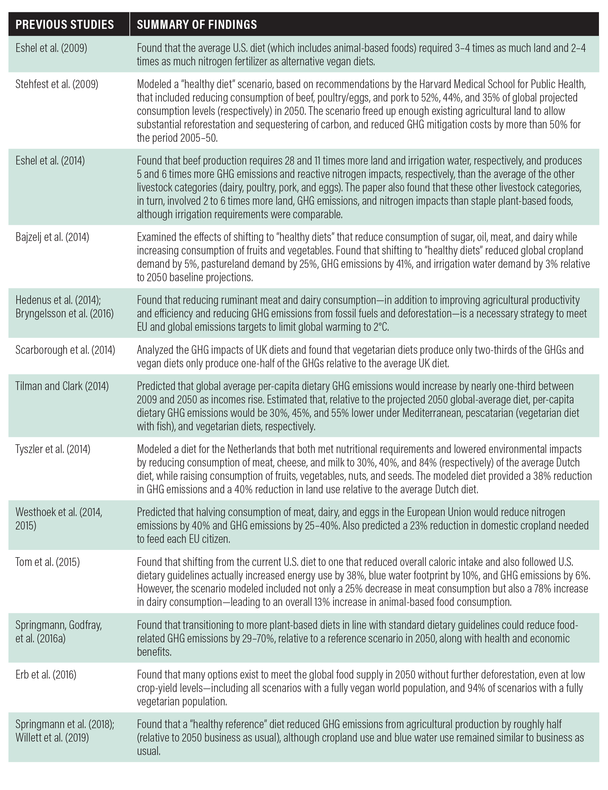
Table B-1 summarizes papers that examine the implications of reducing meat and dairy consumption in diets. They have consistently found large reductions in land use and GHG emissions, although effects on water use can depend on the level of fruit, vegetable, and nut consumption. Because each of the studies discussed in this list uses a different approach, and because some include GHG emissions from food processing and retail and not merely production-related emissions at the farm, their results are not directly comparable to each other or to GlobAgri results.

The GlobAgri-WRR model builds on previous studies and addresses some of their limitations. Many other studies are based not on one consistent model but on average results from multiple lifecycle assessments performed by different researchers of different foods. This approach can introduce inconsistencies due to the widely varying methods and assumptions of different lifecycle assessments. Moreover, some modeling analyses, such as Eshel et al. (2014), focus only on one country. GlobAgri-WRR applies a single modeling approach to production of foods throughout the world. It is most similar in basic approach to Bajzelj et al. (2014) and Hedenus et al. (2014). A principal difference is that GlobAgri-WRR is substantially more disaggregated. It can therefore estimate, for example, not just broad global shifts in diets, but diet shifts only in regions where people consume large quantities of animal-based foods. It can also examine the regional consequences of these shifts and interactions with more possible changes in production methods.

Table B-1 |

Summary of findings by previous studies examining the implications of shifting toward lower meat and dairy consumption